JPEG from Zero to Hero: How JPEG Compression Works, Its Variants, and an Encoder You Build in Python

In short: We follow one espresso photo through JPEG. Part 1 tells the story of how JPEG compression works: what it keeps, what it quietly throws away, and why your eyes don’t notice. Part 2 meets the rest of the family, from progressive JPEG to JPEG XL and JPEG AI, measured on the same photo. Part 3 is the tutorial: you build a baseline JPEG encoder in about 350 lines of Python that writes real .jpg files and lands within 1% of libjpeg-turbo’s file size.

Here is a photo of an espresso, sitting on a worn wooden table. It is 600 pixels wide and 400 tall, and every pixel is three numbers: how much red, green and blue it holds. That is 720,000 bytes.

Save it as a JPEG at quality 75, the default in libjpeg and Pillow, and it shrinks to 40,908 bytes, seventeen times smaller. Put the two side by side and you will struggle to say which is which.

That should feel slightly suspicious. Nearly 680,000 bytes have gone, and you can’t see where. This article is the story of where they went. First we follow the photo through JPEG one step at a time, then we meet the formats that grew out of it, and finally you write an encoder that does the whole journey yourself.

Part 1: How JPEG compression works

JPEG doesn’t store your photo. It stores what you will notice.

JPEG was designed in the late 1980s, when sending our espresso photo over a 2,400 bits-per-second modem would have taken 40 minutes. A lossless squeeze, the kind ZIP or PNG does, saves only about 40% on a photo like this, because photos are full of fine noise that never repeats exactly. So the committee behind JPEG asked a different question: not “how do we store every pixel?” but “which parts of this picture would a person actually miss?”

The answer came from two habits of the human eye, and the whole format is built on them.

Your eye cares more about brightness than about colour. You notice a slight change in how light or dark something is far more easily than a slight change in its hue, especially in small details.

Your eye cares more about broad shapes than about fine texture. The curve of the cup matters to you; the exact grain of the wood under it, much less.

Keep those two habits in mind. Every step that follows exploits one of them.

Step 1: Split brightness from colour

A camera records red, green and blue, but those three mix brightness and colour together. So JPEG first rewrites each pixel as three different numbers: Y, the brightness (called luma), and two colour numbers, Cb (how blue it is) and Cr (how red it is). Nothing is lost yet; it is the same information, sorted differently.

Look at what that does to our photo:

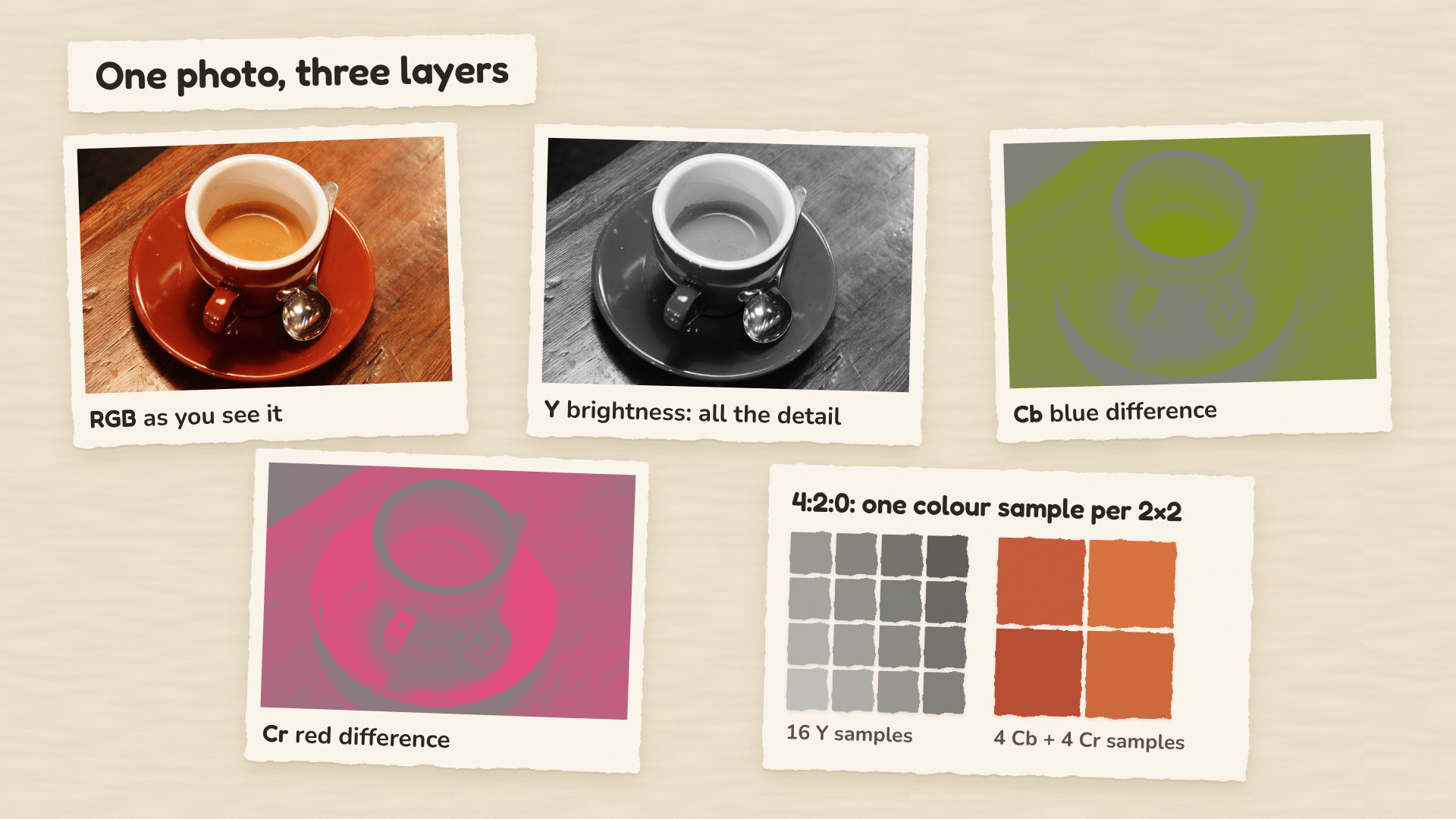
All the detail lives in Y: the crema, the wood grain, the reflections in the spoon. The two colour layers are soft, almost blurry.

Step 2: Keep less colour

Since your eye barely uses colour detail, JPEG stores the colour layers at a lower resolution. The usual choice, called 4:2:0, keeps one colour sample for every 2×2 square of pixels, so each colour layer shrinks to a quarter of its size.

This is the first step that loses information, and on a photo it is almost free: our three full layers become one full layer plus two quarter layers, half the numbers we started with.

Step 3: Describe each tile as a mix of patterns

Now JPEG cuts each layer into tiles of 8×8 pixels and does something that sounds odd. Instead of storing the 64 pixel values of a tile, it describes the tile as a mix of 64 fixed patterns, from a perfectly flat square to a fine checkerboard, and stores how much of each pattern the tile needs.

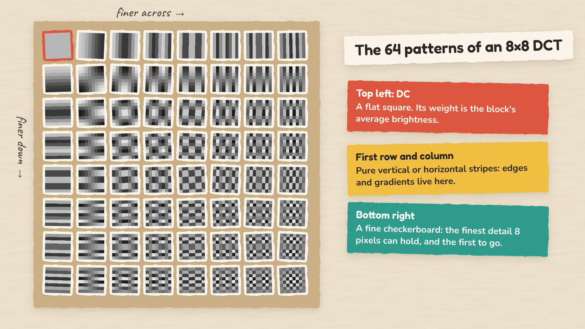
This rewrite is the discrete cosine transform, the DCT. Any 8×8 tile is exactly some mix of these patterns, so nothing is lost. What changes is the order of things. Most tiles in a photo are mostly smooth, so most of their information lands on the few coarse patterns at the top left, and the fine patterns get tiny weights.

Watch it happen on one real tile, taken from the rim of the cup. The animation adds the patterns one at a time, coarse to fine:

A handful of patterns already give you the edge and the shading. Everything after that is fine texture, the part your eye cares least about. That is the opening JPEG needs.

Step 4: Round the weights (this is the quality slider)

Here is where JPEG throws information away on purpose. It divides each pattern’s weight by a step size and rounds the result to a whole number. Coarse patterns get small steps, so they are kept accurately. Fine patterns get large steps, so their small weights round to zero.

The 64 step sizes form the quantisation table, and the quality setting in your image library simply scales that table up or down. Quality 90 means small steps and little rounding. Quality 10 means huge steps, and most of every tile rounds to nothing. When you type quality=85, this is the knob you are turning.

Step 5: Pack what’s left

After rounding, most weights in most tiles are zero. JPEG reads each tile in a zig-zag from coarse to fine patterns, so the zeros pile up at the end, where a single “end of tile” symbol can stand in for all of them. Then Huffman coding gives the most common symbols the shortest bit codes, the same idea as Morse code giving the letter E a single dot.

Here is the whole journey in numbers for our photo at quality 75:

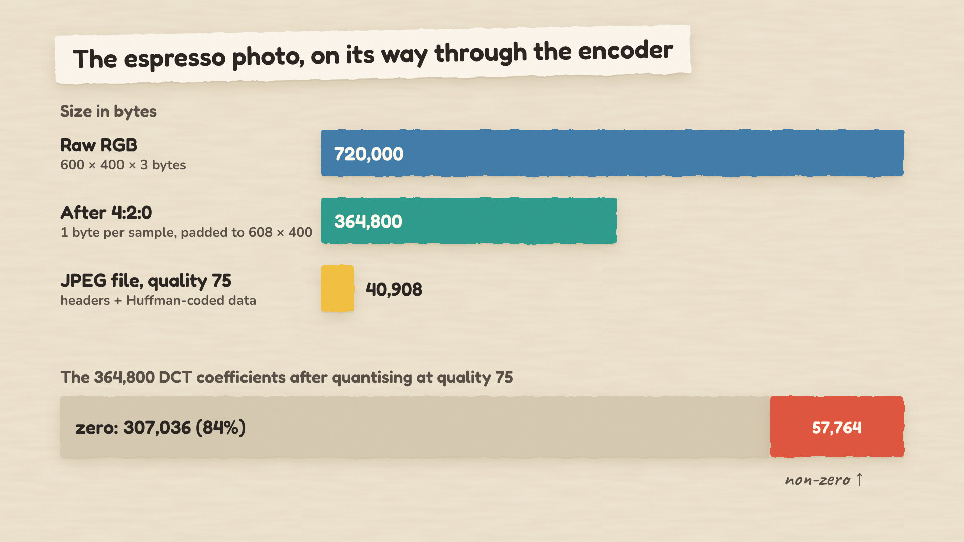
The bottom strip is the whole trick in one picture. After rounding, 84% of the numbers are zero, and zeros cost almost nothing to store.

The way back

Opening a JPEG runs the journey in reverse: unpack the symbols, multiply the weights back up, turn the patterns back into pixels, enlarge the colour layers and convert to red, green and blue. Only two steps can’t be undone, because they threw something away: shrinking the colour in step 2 and rounding in step 4. Everything else comes back exactly.

How far can you push it? A 1991 description of the standard by Gregory Wallace, who chaired the committee, gave a rough guide for colour photos: 0.25 to 0.5 bits per pixel for moderate to good quality, 0.75 to 1.5 for excellent, and 1.5 to 2 for results usually indistinguishable from the original. Our quality 75 file works out at 1.36 bits per pixel.

Where JPEG breaks

Once you know the journey, you can predict where it goes wrong:

• Text, line art and screenshots. Sharp edges need lots of fine patterns, exactly what rounding removes, so every letter grows a faint ripple and coloured text smears. PNG or WebP lossless are better tools here.
• Transparency. The classic JPEG has no alpha channel.
• Very low quality. When nearly every fine weight rounds away, each tile collapses to its flat average and the 8×8 grid shows through.
• Editing loops. Every save rounds again, against a tile grid that shifts when you crop. Part 3 measures how much that costs.

Part 2: The JPEG family

“JPEG” today means more than one format. The 1992 standard has hidden modes most people never meet, a set of wrappers that carry metadata, better encoders that still write the same format, and a line of successors. Here is the whole family tree at a glance:

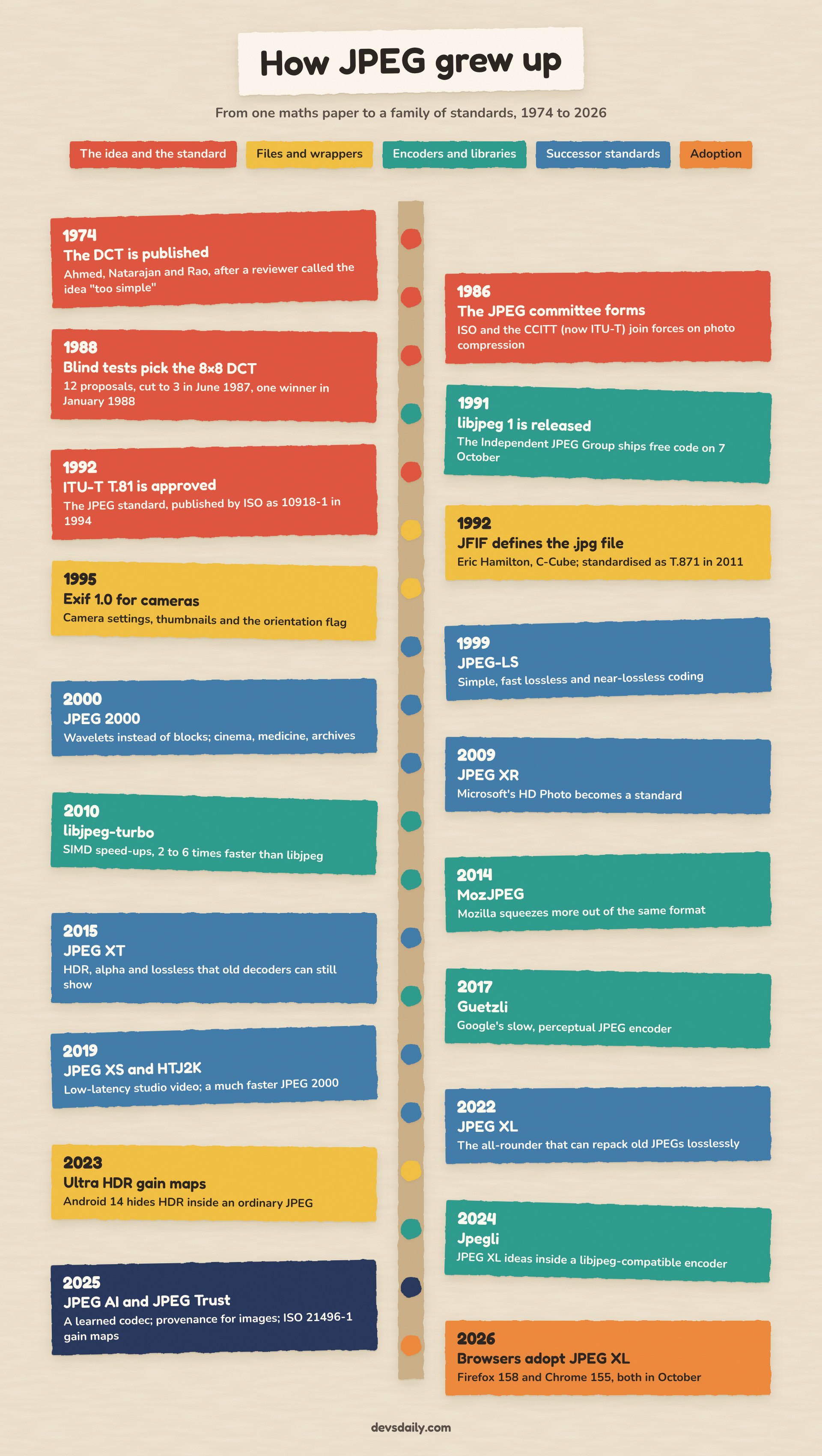
Two moments on that timeline shape everything below. The free libjpeg code of 1991 is a big reason JPEG ended up on every device, and the patents on one optional part of the 1992 standard are the reason a better coder sat unused for thirty years. You will meet both in a moment.

Inside the 1992 standard: the modes

The standard describes more than the JPEG you know:

Mode	What changes	Where you meet it
Baseline	8-bit samples, Huffman coding, one top-to-bottom pass	Almost every .jpg you have opened
Extended	Adds 12-bit samples and arithmetic coding	Medical and scientific imaging
Progressive	The same data, sent in passes from coarse to fine	Web images, if the encoder chooses it
Lossless	No DCT; predicts each pixel from its neighbours	Some medical images and camera raw files
Hierarchical	Several resolutions, each refining the last	Almost nowhere; libjpeg never implemented it

I encoded the espresso photo in each mode today’s libraries support, at quality 75 (the scripts behind every number in this part are in the appendix):

Variant	Size	Change
Baseline, the standard’s typical Huffman tables	41,606 B
Baseline, Huffman tables tuned to this photo	40,865 B	-1.8%
Progressive	40,493 B	-2.7%
Arithmetic coding, same data repacked	38,289 B	-8.0%
Lossless mode	467,544 B	11 times bigger, but exact

Progressive JPEG stores exactly the same rounded weights, just in a different order. A baseline file is stored tile by tile from top to bottom, so a slow download paints the picture like a roller blind. A progressive file sends the average of every tile first, then the coarse patterns, then the fine ones, so you see a blurry version of the whole photo almost at once. This animation decodes the real bytes of both files as they arrive:

libjpeg-turbo split our photo into ten passes. After the first 9% of the file you have the whole picture at 22.95 dB, and after a third of it 28.03 dB. When the last pass lands, the pixels match the baseline file exactly.

Arithmetic coding is the road not taken. It saved 8.0% for free, with identical pixels, yet almost nobody uses it. In the 1990s it was covered by patents; the Independent JPEG Group removed it from libjpeg and warned that it “cannot legally be used without obtaining one or more licenses”. The patents have long since expired, but thirty years of software grew up without it. That history still bites: in Chromium 153 (the build bundled with Playwright), arithmetic-coded and 12-bit files report a successful decode and then draw a completely transparent image. There is no error to catch; your users just see nothing.

Around the image data: the wrappers

A .jpg file is a list of tagged segments, and decoders skip the segments they don’t understand. That one design choice let people add features for thirty years without breaking old viewers:

• JFIF (1992) says which colour space the numbers use; it is what made .jpg files interchangeable.
• Exif (1995) carries camera settings, GPS, a thumbnail and the orientation flag. If you strip metadata from uploads, rotate the pixels first (in Pillow, ImageOps.exif_transpose), or portrait photos come out sideways.
• ICC profiles describe exactly what the colour numbers mean, for wide-gamut screens and print.
• Gain maps hide an HDR version inside an ordinary JPEG. Android 14 introduced Ultra HDR in 2023, and ISO 21496-1 standardised the metadata in 2025; old viewers just show the normal picture.

Same format, smarter encoders

The standard fixes what a decoder must do but leaves the encoder free to choose its tables and its rounding. So encoders kept improving without anyone else changing anything. libjpeg-turbo (2010) made the original library 2 to 6 times faster, by its maintainers’ measure, and it now sits inside most browsers and Android. Mozilla’s MozJPEG (2014), Google’s Guetzli (2017) and Google’s jpegli (2024) all produce ordinary JPEGs that are smaller at the same visual quality; Google reported about 35% for both of its encoders, on its own tests and, for jpegli, at high quality settings. If you serve a lot of JPEGs, switching the encoder is the cheapest saving available.

The successors

The committee kept going where JPEG could not stretch:

• JPEG-LS (1999): simple, fast lossless and near-lossless coding.
• JPEG 2000 (2000): wavelets instead of 8×8 tiles, so no blocking; it became the format of digital cinema and many medical and archive systems.
• JPEG XR (2009): Microsoft’s HD Photo, with HDR and alpha; it never spread far beyond Windows.
• JPEG XT (2015): HDR, alpha and lossless as extensions that old JPEG decoders can still show.
• JPEG XS (2019): not for files but for live video in broadcast studios, with a delay of only a few lines of pixels.
• JPEG XL (2022): the modern all-rounder, which can also repack an existing JPEG into a smaller file and restore the original bytes exactly.
• JPEG AI (2025): the first where the transform is a trained neural network.

Here is how they compare on our photo. First, lossless compression, where every file decodes back to exactly the original pixels:

Format	Size	Ratio
Lossless JPEG (1992)	467,544 B	1.54:1
PNG	441,801 B	1.63:1
JPEG-LS	388,935 B	1.85:1
JPEG XR	383,569 B	1.88:1
JPEG 2000	356,911 B	2.02:1
WebP lossless	336,030 B	2.14:1
JPEG XL	335,090 B	2.15:1

Thirty years of work bought about 28% over the 1992 lossless mode. Photos are noisy, and noise can’t be squeezed losslessly, which is exactly why JPEG chose to be lossy.

JPEG XL’s repacking trick did better than any of these on its own terms: it turned our 41,606 byte JPEG into a 36,041 byte JPEG XL file, 13.4% smaller, and decoding it gave back the original JPEG byte for byte.

Then lossy compression. I tuned each encoder to produce a file the same size as our quality 75 JPEG and measured the result (WebP and AVIF are not JPEG standards, but you will be choosing between them):

Format	Size	PSNR	SSIM
JPEG (1992)	40,865 B	32.43 dB	0.9083
JPEG XL	40,814 B	33.77 dB	0.9265
JPEG XR	40,851 B	34.79 dB	0.9326
WebP	40,320 B	34.92 dB	0.9360
JPEG 2000	40,856 B	35.73 dB	0.9352
AVIF	39,914 B	36.84 dB	0.9542

PSNR and SSIM compare pixel values, and higher is better for both. Take the ranking with a pinch of salt: it is one photo, and the encoders aim at different targets (JPEG 2000’s encoder here maximises PSNR directly, while JPEG XL’s is tuned for how people see, which pixel metrics undervalue). The safe conclusion is the headline: at the same size, every successor beats the 1992 format clearly.

And yet the 1992 format is still everywhere, because formats spread through decoders, not encoders. My Chromium 153 test decoded WebP and AVIF but none of JPEG-LS, JPEG 2000, JPEG XR or JPEG XL. That is finally changing for JPEG XL: Safari has decoded it since version 17 (caniuse marks the support as partial), and Firefox 158 and Chrome 155 both turned it on in October 2026. When I wrote this, caniuse showed no Edge version with it enabled, so serve JPEG XL with a JPEG fallback in a <picture> element.

JPEG AI: when the patterns are learned

Every format so far uses patterns designed by people. JPEG AI, published in September 2025 as ISO/IEC 6048-1, replaces them with a trained neural network. The journey from Part 1 maps across almost step for step:

Classic JPEG	JPEG AI
Fixed 64 DCT patterns per 8×8 tile	A trained network turns the whole image into a compact “latent”
Quantisation table	Rounding of the latent, with a learned gain to control quality, even region by region
Huffman codes	Entropy coding driven by probabilities a second small network predicts
Inverse DCT	A trained network rebuilds the pixels

Learned patterns can describe textures and edges far better than 64 fixed cosines, so the same quality needs fewer bits. The committee describes roughly a 30% saving over the best conventional codecs at the same subjective quality, and an overview paper by Esenlik and colleagues (IEEE TCSVT, 2026) measures 14% to 27% against VVC Intra, the still-image mode of the H.266 video codec, depending on which encoder and decoder are used. The costs are compute and caution: decoding runs neural networks (the standard defines three decoders, from about 14 to 215 thousand multiply-accumulates per pixel, all reading the same file), and the paper notes weaker results on screenshots with text.

When I wrote this, no browser decoded JPEG AI, so it is not a web format yet. It makes sense where you control both ends, such as photo archives and camera-to-cloud pipelines, and the reference software is linked from jpeg.org if you want to measure it on your own images.

Choosing a format today

You are storing	Reach for
Photos for the web, maximum compatibility	JPEG from a good encoder (MozJPEG or jpegli), progressive
Photos for the web, smaller files	AVIF or JPEG XL, with a JPEG fallback in <picture>
An existing JPEG archive you want smaller	JPEG XL lossless repacking
Screenshots, diagrams, text	PNG or WebP lossless, or JPEG with 4:4:4 colour if it must be JPEG
Medical, cinema, archive masters	JPEG 2000 or a lossless format
A closed pipeline where compression matters most	Evaluate JPEG AI on your own images

Part 3: Build a JPEG encoder in Python

Reading about the journey is one thing; making it happen is another. In this part you write the five steps from Part 1 as code, ending with a real .jpg file that any viewer opens.

All the encoder code goes into one file, tinyjpeg.py. Each code block in this part is the next piece of that file, so paste them in order. It needs only NumPy; Pillow and scikit-image are for testing it.

Colour: from RGB to YCbCr

These are the full-range formulas from JFIF (ITU-T T.871), which nearly every JPEG decoder assumes. The weights in the Y line reflect how bright each primary looks to us; green counts for almost 60%.

"""tinyjpeg: a baseline JPEG encoder in plain Python + NumPy, written to be read.

It writes real .jpg files (baseline DCT, 4:2:0, optimised Huffman tables)
that any image viewer can open. It is slow and skips every speed trick on purpose.
"""
import heapq
import struct

import numpy as np


def rgb_to_ycbcr(rgb):
    """JFIF full-range conversion. Input uint8 HxWx3, output float HxWx3."""
    rgb = rgb.astype(np.float64)
    r, g, b = rgb[..., 0], rgb[..., 1], rgb[..., 2]
    y = 0.299 * r + 0.587 * g + 0.114 * b
    cb = -0.168736 * r - 0.331264 * g + 0.5 * b + 128
    cr = 0.5 * r - 0.418688 * g - 0.081312 * b + 128
    return np.stack([y, cb, cr], axis=-1)


def ycbcr_to_rgb(ycc):
    y, cb, cr = ycc[..., 0], ycc[..., 1] - 128, ycc[..., 2] - 128
    r = y + 1.402 * cr
    g = y - 0.344136 * cb - 0.714136 * cr
    b = y + 1.772 * cb
    return np.clip(np.round(np.stack([r, g, b], axis=-1)), 0, 255).astype(np.uint8)

The conversion is a 3×3 matrix and an offset, and the decoder runs the inverse, so nothing is lost here beyond rounding.

Chroma subsampling: the first lossy step

def pad_to_multiple(plane, m):
    """Repeat the last row/column until both sides are a multiple of m."""
    h, w = plane.shape
    return np.pad(plane, ((0, (-h) % m), (0, (-w) % m)), mode="edge")


def downsample_2x2(plane):
    """4:2:0 chroma: average each 2x2 square into one sample."""
    h, w = plane.shape
    return plane.reshape(h // 2, 2, w // 2, 2).mean(axis=(1, 3))


def upsample_2x2(plane):
    return plane.repeat(2, axis=0).repeat(2, axis=1)

JPEG cuts planes into whole blocks, so we pad every plane by repeating its edge. With 4:2:0 the encoder works in 16×16 pixel units, so our 600×400 photo is padded to 608×400. The decoder knows the real size from the header and crops the padding off.

How much does subsampling buy? With Pillow at quality 75, keeping full-resolution colour (4:4:4) gives a 51,481 byte file at 33.41 dB PSNR. With 4:2:0 the file drops to 40,865 bytes at 32.43 dB: 21% smaller for a loss you would struggle to spot in a photo. For screenshots with thin coloured text it is a bad deal; ask your library for 4:4:4. Every figure in this article is a JPEG saved with 4:4:4 for exactly that reason: they are full of text.

The DCT in code

The DCT is a single 8×8 matrix. Row k of that matrix is the k-th cosine pattern in one dimension, and multiplying on both sides applies it to the rows and the columns of a block:

def dct_matrix(n=8):
    """Row k is the k-th cosine basis vector, scaled so the matrix is orthonormal."""
    c = np.zeros((n, n))
    for k in range(n):
        alpha = np.sqrt(1 / n) if k == 0 else np.sqrt(2 / n)
        for x in range(n):
            c[k, x] = alpha * np.cos((2 * x + 1) * k * np.pi / (2 * n))
    return c


C = dct_matrix()


def dct2(block):
    return C @ block @ C.T


def idct2(coeffs):
    return C.T @ coeffs @ C

The matrix is orthonormal, so its transpose is its inverse; that is why idct2 is the same expression with C.T and C swapped. Before the transform, JPEG subtracts 128 from every sample so values sit around zero.

Let’s watch a real block: the same tile from the cup’s rim that the animation in Part 1 rebuilt. Save this next to tinyjpeg.py as one_block.py. It uses functions from the next three sections, so run it once tinyjpeg.py is complete; I show its output in two halves as we go.

import numpy as np
from skimage import data

import tinyjpeg as tj

np.set_printoptions(linewidth=120, suppress=True)

rgb = data.coffee()
y = tj.rgb_to_ycbcr(rgb)[..., 0]
block = y[96:104, 264:272]                 # 8x8 on the cup's inner rim

print("pixels (Y):\n", np.round(block).astype(int))
coeffs = tj.dct2(block - 128)
print("DCT coefficients:\n", np.round(coeffs).astype(int))
table = tj.scale_table(tj.LUMA_Q, 75)
q = tj.quantize(coeffs, table)
print("quantised (q=75):\n", q)
zz = tj.to_zigzag(q)
print("zig-zag:", zz.tolist())
dc, ac = tj.block_symbols(zz, prev_dc=0)
print("symbols:", [(hex(s), b, n) for s, b, n in dc + ac])
back = tj.idct2(tj.dequantize(q, table)) + 128
print("decoded pixels:\n", np.round(back).astype(int))
print("max pixel error:", int(np.abs(np.round(back) - np.round(block)).max()))

The first half of what it prints:

pixels (Y):
 [[133 124 128 126 129 119 117 118]
 [105  92  94  94  98  94  95 102]
 [ 92  93  96  96  92  96  97  96]
 [ 93  91  93  93  91  91  95  96]
 [ 91  90  88  87  80  87  91  85]
 [ 81  91  83  82  76  76  84  77]
 [ 83  84  83  80  80  81  73  81]
 [ 76  72  79  75  75  77  77  80]]
DCT coefficients:
 [[-290    7    5   -3    1    3    2    1]
 [  97    2   -1    3    8    1    1    4]
 [  27    3   -3    2    8   -4    6    4]
 [  29   14    0    1   -2    0   -5    0]
 [  27    0   -1    1    1    3    1    2]
 [  26    4   -6   -1    1   -4    0   -1]
 [   9    0   -4   -3   -7    2   -5    0]
 [   8    2   -2    2   -2    0    3   -2]]

The top row of pixels is brighter than the rest, and brightness fades downward. That is a horizontal edge, and the DCT says so: the big values sit in the first column, which holds the patterns with horizontal stripes. The -290 in the corner is the DC coefficient, eight times the block’s average after the level shift. Most other entries are single digits.

Quantisation: where the quality slider lives

The JPEG standard’s Annex K gives example quantisation tables, tuned on how visible each pattern is to people. They are not mandatory, but nearly every encoder starts from them. The quality number you pass to a library is not part of the standard at all. It is libjpeg’s convention for scaling these tables: quality 50 uses them as printed, lower values multiply them up, higher values shrink them, and 100 sets every step to 1.

# Example tables from Annex K of the JPEG standard (ITU-T T.81), in row order.
LUMA_Q = np.array([
    16, 11, 10, 16, 24, 40, 51, 61,
    12, 12, 14, 19, 26, 58, 60, 55,
    14, 13, 16, 24, 40, 57, 69, 56,
    14, 17, 22, 29, 51, 87, 80, 62,
    18, 22, 37, 56, 68, 109, 103, 77,
    24, 35, 55, 64, 81, 104, 113, 92,
    49, 64, 78, 87, 103, 121, 120, 101,
    72, 92, 95, 98, 112, 100, 103, 99]).reshape(8, 8)

CHROMA_Q = np.array([
    17, 18, 24, 47, 99, 99, 99, 99,
    18, 21, 26, 66, 99, 99, 99, 99,
    24, 26, 56, 99, 99, 99, 99, 99,
    47, 66, 99, 99, 99, 99, 99, 99,
    99, 99, 99, 99, 99, 99, 99, 99,
    99, 99, 99, 99, 99, 99, 99, 99,
    99, 99, 99, 99, 99, 99, 99, 99,
    99, 99, 99, 99, 99, 99, 99, 99]).reshape(8, 8)


def scale_table(base, quality):
    """The libjpeg quality formula: 50 uses the table as-is, 100 makes every entry 1."""
    quality = min(max(quality, 1), 100)
    scale = 5000 // quality if quality < 50 else 200 - 2 * quality
    table = (base * scale + 50) // 100
    return np.clip(table, 1, 255).astype(np.int32)


def quantize(coeffs, table):
    return np.round(coeffs / table).astype(np.int32)


def dequantize(q, table):
    return q * table

The luma table runs from 16 in the top left to 121 near the bottom right, so fine checkerboard detail is divided by steps roughly seven times larger than the one used for the block average. The chroma table is even harsher; it is mostly 99.

Back to our rim block. The second half of the output shows it after quantising at quality 75, and then after the decoder multiplies back and runs the inverse DCT:

quantised (q=75):
 [[-36   1   1   0   0   0   0   0]
 [ 16   0   0   0   1   0   0   0]
 [  4   0   0   0   0   0   0   0]
 [  4   2   0   0   0   0   0   0]
 [  3   0   0   0   0   0   0   0]
 [  2   0   0   0   0   0   0   0]
 [  0   0   0   0   0   0   0   0]
 [  0   0   0   0   0   0   0   0]]
zig-zag: [-36, 1, 16, 4, 0, 1, 0, 0, 0, 4, 3, 2, 0, 0, 0, 0, 1, 0, 0, 0, 2, 0, 0, ...]
symbols: [('0x6', 27, 6), ('0x1', 1, 1), ('0x5', 16, 5), ('0x3', 4, 3), ('0x11', 1, 1), ('0x33', 4, 3), ('0x2', 3, 2), ('0x2', 2, 2), ('0x41', 1, 1), ('0x32', 2, 2), ('0x0', 0, 0)]
decoded pixels:
 [[131 125 123 125 124 118 117 121]
 [102  98  97 101 101  97  98 102]
 [ 91  88  89  92  93  92  94  98]
 [ 95  94  93  94  95  95  96  98]
 [ 91  90  89  86  85  85  85  84]
 [ 86  87  85  80  78  79  78  76]
 [ 82  85  84  79  78  82  82  79]
 [ 73  77  77  73  74  80  82  78]]
max pixel error: 9

Fifty-four of the 64 values are now zero. The decoded block keeps the edge and the overall shading, but the pixel-level texture is gone; the worst pixel is off by 9 out of 255. Across the whole photo at quality 75, 79% of luma coefficients and about 94% of chroma coefficients end up zero.

Zig-zag order and run-length symbols

def zigzag_order(n=8):
    """(row, col) pairs walking the anti-diagonals, alternating direction."""
    order = []
    for s in range(2 * n - 1):
        diag = [(i, s - i) for i in range(n) if 0 <= s - i < n]
        order.extend(diag if s % 2 else diag[::-1])
    return order


ZIGZAG = zigzag_order()
ZZ_ROWS = np.array([r for r, _ in ZIGZAG])
ZZ_COLS = np.array([c for _, c in ZIGZAG])


def to_zigzag(block):
    return block[ZZ_ROWS, ZZ_COLS]

Each block then becomes a short list of symbols:

• The DC value is stored as the difference from the previous block’s DC in the same channel, because neighbouring blocks usually have similar averages. Our rim block’s DC is -36 and the block before it had -29, so the encoder stores -7.
• Each non-zero AC value becomes one byte-sized symbol that packs two things: how many zeros came before it (the run, 0 to 15) and how many bits its value needs (the size). The value itself follows as size raw bits.
• EOB (end of block, symbol 0x00) says “everything after this is zero”.
• ZRL (0xF0) stands for 16 zeros in a row, for the rare run longer than 15.

Negative values use a trick worth knowing. A value of size s is stored in s bits; positive values are written as is, and negative values as v + 2^s - 1. So 5 is 101 and -5 is 010, its bitwise complement. The size already tells the decoder the magnitude range, so the leading bit is enough to tell the sign.

def size_and_bits(v):
    """JPEG's (category, extra bits) for a value. Negative values store v - 1 in 'size' bits."""
    if v == 0:
        return 0, 0
    size = int(abs(v)).bit_length()
    bits = v if v > 0 else v + (1 << size) - 1
    return size, bits


def block_symbols(zz, prev_dc):
    """Turn one zig-zagged block into (huffman_symbol, extra_bits, n_extra) tuples."""
    dc_diff = int(zz[0]) - prev_dc
    size, bits = size_and_bits(dc_diff)
    dc = [(size, bits, size)]

    ac, run = [], 0
    last_nonzero = max((i for i in range(1, 64) if zz[i] != 0), default=0)
    for i in range(1, last_nonzero + 1):
        v = int(zz[i])
        if v == 0:
            run += 1
            continue
        while run > 15:               # ZRL: a run of 16 zeros
            ac.append((0xF0, 0, 0))
            run -= 16
        size, bits = size_and_bits(v)
        ac.append(((run << 4) | size, bits, size))
        run = 0
    if last_nonzero < 63:
        ac.append((0x00, 0, 0))      # EOB: the rest of the block is zero
    return dc, ac

In the output above, ('0x33', 4, 3) means “3 zeros, then a value that needs 3 bits, and those bits are 4”. The prev_dc=0 in the script is only for display; inside a real file this block’s DC difference is -7.

Huffman coding with JPEG’s two extra rules

JPEG keeps four Huffman tables: one DC and one AC table for luma, the same pair for chroma. The standard ships typical tables, but an encoder may build tables tuned to the image and store them in the file. Pillow does this when you pass optimize=True, and so do we. Two rules make it slightly more than textbook Huffman: no code may be longer than 16 bits, and no code may consist only of 1 bits. Padding at the end of the data is made of 1 bits, so this keeps a decoder from reading padding as a symbol.

The code below follows the method in Annex K.3 of the standard, which is also what libjpeg does. A dummy symbol with count 1 claims the all-ones code during construction and is dropped afterwards. If any code ends up longer than 16 bits, the loop shortens codes in pairs while keeping the code set complete.

def huffman_code_lengths(freqs):
    """Classic Huffman on a {symbol: count} dict. Returns {symbol: code_length}."""
    heap = [(f, i, [s]) for i, (s, f) in enumerate(freqs.items())]
    heapq.heapify(heap)
    lengths = {s: 0 for s in freqs}
    if len(heap) == 1:
        return {s: 1 for s in freqs}
    tie = len(heap)
    while len(heap) > 1:
        f1, _, s1 = heapq.heappop(heap)
        f2, _, s2 = heapq.heappop(heap)
        for s in s1 + s2:
            lengths[s] += 1
        heapq.heappush(heap, (f1 + f2, tie, s1 + s2))
        tie += 1
    return lengths


def build_jpeg_table(freqs):
    """Optimal table with JPEG's rules: max 16 bits, and no code made only of 1s.

    Returns (bits, huffval) as stored in a DHT segment, and a {symbol: (code, length)} map.
    """
    freqs = dict(freqs)
    freqs[256] = 1                      # dummy symbol reserves the all-ones code
    lengths = huffman_code_lengths(freqs)

    bits = [0] * (max(max(lengths.values()), 16) + 1)   # bits[n] = how many codes of length n
    for s, n in lengths.items():
        bits[n] += 1
    # Annex K.3: move symbols out of lengths > 16 while keeping the code complete.
    for i in range(len(bits) - 1, 16, -1):
        while bits[i] > 0:
            j = i - 2
            while bits[j] == 0:
                j -= 1
            bits[i] -= 2
            bits[i - 1] += 1
            bits[j + 1] += 2
            bits[j] -= 1
    i = 16
    while bits[i] == 0:
        i -= 1
    bits[i] -= 1                        # drop the dummy symbol's slot

    # Shortest original codes first, ties broken by symbol value (as libjpeg does).
    huffval = sorted((s for s in lengths if s != 256), key=lambda s: (lengths[s], s))

    codes, code, k = {}, 0, 0
    for length in range(1, 17):
        for _ in range(bits[length]):
            codes[huffval[k]] = (code, length)
            code += 1
            k += 1
        code <<= 1
    return bits[1:17], huffval, codes

On the coffee photo, at the qualities used here, that length-limiting loop never runs; the longest code a plain Huffman tree produces is at most 16 bits. To make sure it works, the tests at the end of this part feed it counts of 3^0, 3^1, 3^2 and so on for up to 60 symbols, which force trees up to 60 bits deep, and check that every code fits in 16 bits, none is all ones, and none is a prefix of another. An earlier version of this function sized its working array for at most 32-bit trees and crashed on the 33-symbol case; a reviewer caught it, and the array is now sized from the actual tree.

With these tables, our rim block costs 73 bits in the file. Uncompressed, those 64 brightness values were 512 bits.

Writing bits and bytes

Huffman codes are not byte-aligned, so we need a small bit writer. It has one JPEG-specific job. In a JPEG file, a 0xFF byte starts a marker, so whenever the compressed data happens to produce 0xFF, the writer adds a 0x00 after it. The decoder sees FF 00, drops the zero, and carries on. This is called byte stuffing, and forgetting it is the classic bug in a home-made encoder.

class BitWriter:
    def __init__(self):
        self.out = bytearray()
        self.acc = 0
        self.n = 0

    def write(self, value, length):
        for i in range(length - 1, -1, -1):
            self.acc = (self.acc << 1) | ((value >> i) & 1)
            self.n += 1
            if self.n == 8:
                self.out.append(self.acc)
                if self.acc == 0xFF:
                    self.out.append(0x00)   # byte stuffing: 0xFF in data is followed by 0x00
                self.acc, self.n = 0, 0

    def flush(self):
        if self.n:
            self.write((1 << (8 - self.n)) - 1, 8 - self.n)   # pad with 1 bits
        return bytes(self.out)

Putting the pipeline together

forward does everything up to quantisation for all three planes. It uses np.einsum to apply the same C @ block @ C.T to every block at once instead of looping in Python. inverse is the decoder side of the lossy path, which we use to see the damage. mcu_symbols walks the image in the order the file needs: with 4:2:0, each 16×16 area (a minimum coded unit, or MCU) is four Y blocks followed by one Cb and one Cr block.

def split_blocks(plane):
    h, w = plane.shape
    return plane.reshape(h // 8, 8, w // 8, 8).swapaxes(1, 2)   # (rows, cols, 8, 8)


def merge_blocks(blocks):
    r, c = blocks.shape[:2]
    return blocks.swapaxes(1, 2).reshape(r * 8, c * 8)


def forward(rgb, quality):
    """Everything up to (and including) the lossy step. Returns quantised blocks per plane."""
    ycc = rgb_to_ycbcr(rgb)
    y = pad_to_multiple(ycc[..., 0], 16)
    cb = downsample_2x2(pad_to_multiple(ycc[..., 1], 16))
    cr = downsample_2x2(pad_to_multiple(ycc[..., 2], 16))

    qy, qc = scale_table(LUMA_Q, quality), scale_table(CHROMA_Q, quality)
    planes = []
    for plane, table in ((y, qy), (cb, qc), (cr, qc)):
        blocks = split_blocks(plane - 128.0)                  # level shift to -128..127
        coeffs = np.einsum("ij,rcjk,lk->rcil", C, blocks, C)  # dct2 on every block at once
        planes.append(quantize(coeffs, table))
    return planes, (qy, qc)


def inverse(planes, tables, height, width):
    """Decoder side of the lossy path: dequantise, inverse DCT, upsample, back to RGB."""
    qy, qc = tables
    out = []
    for q, table in zip(planes, (qy, qc, qc)):
        coeffs = dequantize(q, table).astype(np.float64)
        pixels = np.einsum("ji,rcjk,kl->rcil", C, coeffs, C) + 128.0   # idct2 per block
        out.append(merge_blocks(pixels))
    y = out[0]
    cb, cr = upsample_2x2(out[1]), upsample_2x2(out[2])
    ycc = np.stack([y, cb, cr], axis=-1)[:height, :width]
    return ycbcr_to_rgb(ycc)


def mcu_symbols(planes):
    """Walk the image in MCUs (4 Y blocks, then Cb, then Cr) and collect symbols."""
    y, cb, cr = planes
    prev = [0, 0, 0]
    stream = []                        # list of (table_kind, symbol, bits, n_bits)
    for mr in range(cb.shape[0]):
        for mc in range(cb.shape[1]):
            units = [(0, y[2 * mr + dr, 2 * mc + dc]) for dr in (0, 1) for dc in (0, 1)]
            units += [(1, cb[mr, mc]), (2, cr[mr, mc])]
            for comp, block in units:
                zz = to_zigzag(block)
                dc, ac = block_symbols(zz, prev[comp])
                prev[comp] = int(zz[0])
                kind = 0 if comp == 0 else 1           # 0 = luma tables, 1 = chroma tables
                stream += [("dc", kind, *dc[0])] + [("ac", kind, *a) for a in ac]
    return stream

The file format

A JPEG file is the list of tagged segments from Part 2. Each segment starts with a two-byte marker (0xFF and a type byte) and, for most segments, a two-byte length. The baseline encoder needs these:

Marker	Bytes	What it carries
SOI	FF D8	Start of image
APP0	FF E0	The JFIF header: version, pixel aspect ratio
DQT	FF DB	A quantisation table, stored in zig-zag order
SOF0	FF C0	Baseline frame: size, components, sampling factors, table choices
DHT	FF C4	A Huffman table: 16 counts of codes per length, then the symbols
SOS	FF DA	Start of scan: which tables each component uses, then the compressed data
EOI	FF D9	End of image

A DHT segment does not store the codes themselves, only how many codes there are of each length and which symbols they belong to. The decoder rebuilds the same canonical codes from that, which is why build_jpeg_table assigns them in a fixed order.

def segment(marker, payload):
    return struct.pack(">HH", marker, len(payload) + 2) + payload


def encode(rgb, quality=75):
    """Return the bytes of a baseline JPEG file."""
    height, width = rgb.shape[:2]
    planes, (qy, qc) = forward(rgb, quality)
    stream = mcu_symbols(planes)

    tables = {}
    for cls in ("dc", "ac"):
        for kind in (0, 1):
            freqs = {}
            for c, k, sym, _, _ in stream:
                if c == cls and k == kind:
                    freqs[sym] = freqs.get(sym, 0) + 1
            tables[cls, kind] = build_jpeg_table(freqs)

    bw = BitWriter()
    for cls, kind, sym, bits, nbits in stream:
        code, length = tables[cls, kind][2][sym]
        bw.write(code, length)
        bw.write(bits, nbits)
    scan = bw.flush()

    out = bytearray(b"\xFF\xD8")                                        # SOI
    out += segment(0xFFE0, b"JFIF\x00\x01\x01\x00\x00\x01\x00\x01\x00\x00")  # APP0
    for tid, table in ((0, qy), (1, qc)):                                # DQT
        out += segment(0xFFDB, bytes([tid]) + bytes(to_zigzag(table).astype(np.uint8)))
    out += segment(0xFFC0, struct.pack(">BHHB", 8, height, width, 3)    # SOF0
                   + bytes([1, 0x22, 0, 2, 0x11, 1, 3, 0x11, 1]))
    for (cls, kind), (bits, huffval, _) in tables.items():               # DHT
        tc = 0 if cls == "dc" else 1
        out += segment(0xFFC4, bytes([(tc << 4) | kind]) + bytes(bits) + bytes(huffval))
    out += segment(0xFFDA, bytes([3, 1, 0x00, 2, 0x11, 3, 0x11, 0, 63, 0]))  # SOS
    out += scan
    out += b"\xFF\xD9"                                                   # EOI
    return bytes(out)


def psnr(a, b):
    mse = np.mean((a.astype(np.float64) - b.astype(np.float64)) ** 2)
    return 10 * np.log10(255 ** 2 / mse)

Here is the file our encoder writes for the coffee photo at quality 75, segment by segment, drawn to scale:

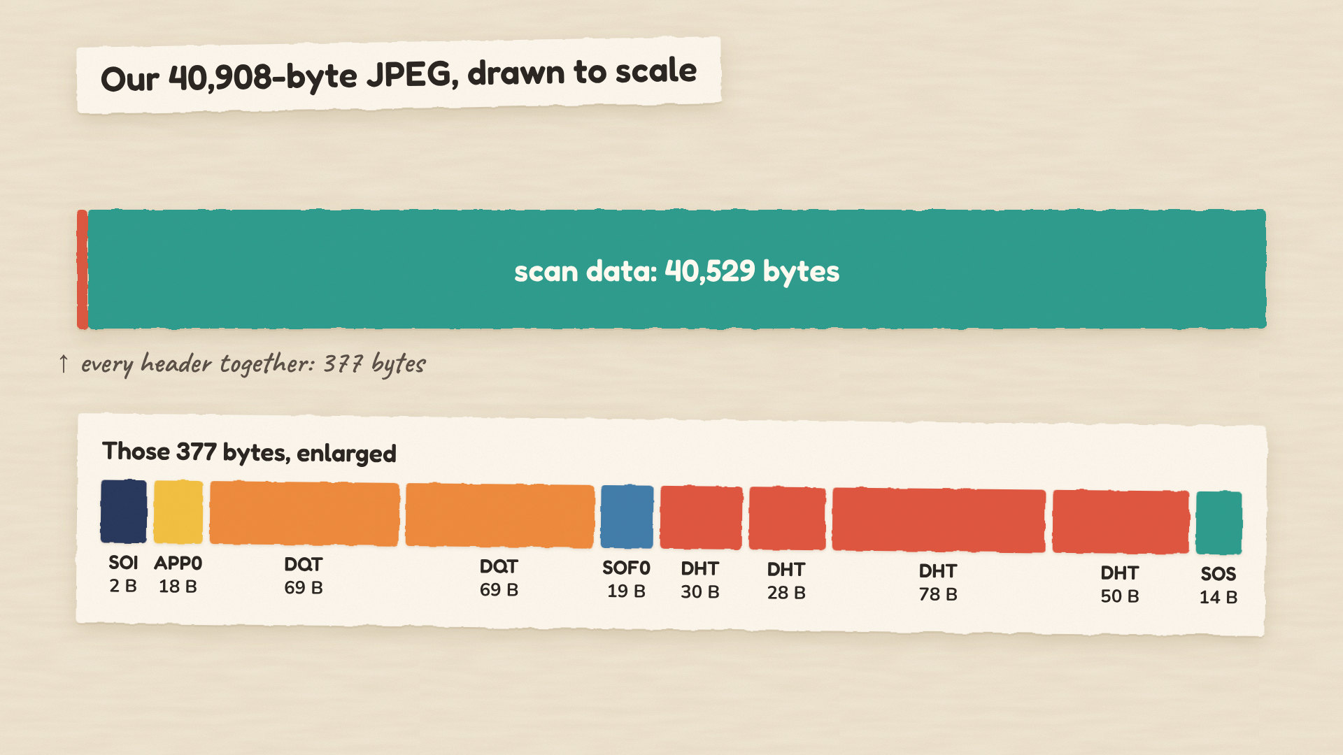
All the structure a decoder needs fits in 377 bytes. Everything else is the scan: the Huffman-coded symbols from the steps above. The sampling bytes in SOF0 are where 4:2:0 is declared: 0x22 gives Y two samples per MCU in each direction, 0x11 gives Cb and Cr one. Change those, the MCU walk and the padding, and you have a 4:4:4 encoder.

Does it work?

Save this as prove_it.py. It writes four files and compares them with Pillow, which uses libjpeg-turbo:

import io

import numpy as np
from PIL import Image
from skimage import data

import tinyjpeg as tj

rgb = data.coffee()

for q in (90, 75, 50, 10):
    ours = tj.encode(rgb, q)
    with open(f"coffee_q{q}.jpg", "wb") as f:
        f.write(ours)

    buf = io.BytesIO()
    Image.fromarray(rgb).save(buf, "JPEG", quality=q, subsampling=2, optimize=True)
    theirs = buf.getvalue()

    ours_px = np.asarray(Image.open(io.BytesIO(ours)).convert("RGB"))
    theirs_px = np.asarray(Image.open(io.BytesIO(theirs)).convert("RGB"))
    print(f"q={q:2d}  tinyjpeg {len(ours):6,d} B  {tj.psnr(rgb, ours_px):.2f} dB   "
          f"Pillow {len(theirs):6,d} B  {tj.psnr(rgb, theirs_px):.2f} dB")

q=90  tinyjpeg 71,136 B  35.53 dB   Pillow 71,303 B  35.51 dB
q=75  tinyjpeg 40,908 B  32.44 dB   Pillow 40,865 B  32.43 dB
q=50  tinyjpeg 26,441 B  30.50 dB   Pillow 26,362 B  30.50 dB
q=10  tinyjpeg  7,635 B  26.03 dB   Pillow  7,588 B  26.03 dB

Every file opens, the sizes are within 0.7% of libjpeg-turbo, and the quality matches to two decimals. That is expected: both encoders use the same tables and the same quality formula, so the remaining gap is small differences in DCT arithmetic, rounding and header bytes. ImageMagick reads our quality 75 file as Quality: 75, estimating it from the quantisation tables alone, and ffmpeg decodes it without errors too.

PSNR (peak signal-to-noise ratio), used throughout this article, compares pixel values with the original; higher is better. There is no universal threshold; how visible the damage is depends heavily on the content, and the same PSNR can look fine on a busy texture and poor on a smooth sky. Sweeping the quality setting shows the classic curve. Size is in bits per pixel, the file size in bits divided by the number of pixels (our quality 75 file is 40,908 × 8 / 240,000 = 1.36 bpp):

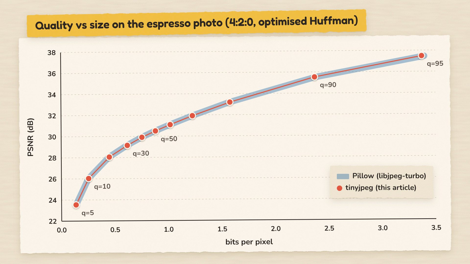
The curve flattens fast. Going from quality 90 to 95 costs 42% more bytes for 2 dB. Going from 10 to 30 more than doubles the size but buys 3 dB that you can clearly see. Most of the useful range for photos sits between 70 and 90.

Two things about our encoder are deliberately simple. It decodes only through Pillow, because a Huffman decoder is the encoder run backwards and makes a good exercise. And inverse upsamples colour by simply repeating each value, while libjpeg-turbo interpolates smoothly, which is why our own reconstruction measures about 0.3 dB lower than Pillow’s decoding of the same file.

Reading JPEG artifacts

Now that you have built every stage, you can read the damage in any JPEG. Here is a crop of the spoon at three quality settings:

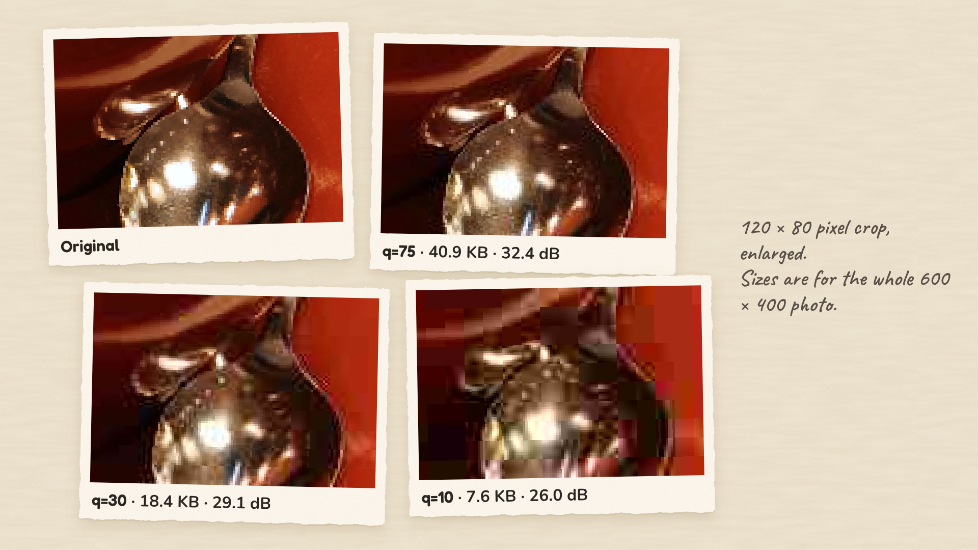
• Blocking is the 8×8 grid showing through at quality 10. Each block is coded on its own, and when almost every AC coefficient rounds to zero, each block collapses to its flat average, so neighbouring blocks no longer join up.
• Ringing is the speckled ripple along the spoon’s right edge, against the red saucer, at quality 30. A sharp edge needs many fine patterns to draw; when quantisation drops some of them, the remaining ones overshoot and undershoot near the edge.
• Colour smearing shows up at quality 10 as purple and pink patches along that same edge, where red saucer meets dark metal. Colour lives at quarter resolution and is quantised hardest, so colour edges blur before brightness edges do.

Saving the same JPEG again and again

A common worry is that every save degrades a JPEG further. This script decodes and re-encodes the coffee photo ten times, first at a fixed quality of 75, then with the quality changing, then with a one-pixel shift before every save:

import io

import numpy as np
from PIL import Image
from skimage import data

from tinyjpeg import psnr


def resave(img, quality):
    buf = io.BytesIO()
    Image.fromarray(img).save(buf, "JPEG", quality=quality, subsampling=2)
    return np.asarray(Image.open(io.BytesIO(buf.getvalue())).convert("RGB"))


original = data.coffee()

img = original
for gen in range(1, 11):
    img = resave(img, 75)
    if gen in (1, 2, 5, 10):
        print(f"generation {gen:2d}: psnr vs original {psnr(original, img):.2f}")

img = original
for gen in range(1, 11):
    img = resave(img, 75 if gen % 2 else 70)
print(f"10 generations alternating q75/q70: {psnr(original, img):.2f}")

img = original
for gen in range(1, 11):
    img = np.roll(resave(img, 75), 1, axis=1)     # shift the block grid by one pixel
img = np.roll(img, -10, axis=1)                    # undo the shifts, then skip the wrapped edges
print(f"10 generations with a 1px shift each: {psnr(original[:, 10:-10], img[:, 10:-10]):.2f}")

generation  1: psnr vs original 32.43
generation  2: psnr vs original 32.33
generation  5: psnr vs original 32.21
generation 10: psnr vs original 32.17
10 generations alternating q75/q70: 30.90
10 generations with a 1px shift each: 26.55

Ten generations lose only 0.26 dB. With the same tables and the same block grid, the second encode finds coefficients that are already close to multiples of the step sizes, so they round back to almost the same values.

That stability breaks easily, though. Alternating between 75 and 70 cost over a decibel more than a single save at 70 (31.92 dB). The one-pixel shift, which is what a crop does to the block grid, ended near what a single quality 10 encode costs (26.03 dB). Re-saving at the same settings is mostly harmless; editing pipelines that crop, rotate by non-multiples of 90 degrees or change quality between saves pile up real damage. Keep the original and export from it.

Where to go from here

You have now taken one photo all the way through JPEG by hand. A few good next steps, if you want to keep going:

• Write the decoder. Read the segments, rebuild the canonical codes from each DHT, and reverse the bit writer and symbol steps. Feed it the files from prove_it.py and compare with Pillow.
• Add 4:4:4 and progressive output. Change the sampling bytes, the padding and the MCU walk for 4:4:4. For progressive, emit the DC scan first and then AC bands, using the scan breakdown that variants.py prints as your guide.
• Try smarter rounding. Rounding to the nearest value is not always the best choice: sending a 0 instead of a 1 can save more bits than it costs in quality. MozJPEG’s trellis quantisation makes those trade-offs with the bit cost in mind. Try a crude version and watch the curve move.

For checking your own changes, here are the tests I used. Save them as test_tinyjpeg.py next to tinyjpeg.py, then run pip install pytest and pytest:

import io

import numpy as np
import pytest
from PIL import Image
from skimage import data

import tinyjpeg as tj


def test_dct_round_trip_is_lossless():
    block = np.random.default_rng(0).uniform(-128, 127, (8, 8))
    assert np.allclose(tj.idct2(tj.dct2(block)), block)


def test_zigzag_starts_like_the_standard():
    assert tj.ZIGZAG[:6] == [(0, 0), (0, 1), (1, 0), (2, 0), (1, 1), (0, 2)]
    assert sorted(tj.ZIGZAG) == [(r, c) for r in range(8) for c in range(8)]


def test_size_and_bits_ones_complement():
    assert tj.size_and_bits(5) == (3, 0b101)
    assert tj.size_and_bits(-5) == (3, 0b010)
    assert tj.size_and_bits(0) == (0, 0)


@pytest.mark.parametrize("n_symbols", [26, 33, 40, 60])
def test_huffman_limits_codes_to_16_bits_and_reserves_all_ones(n_symbols):
    # Counts of 3**s force a maximally skewed tree: plain Huffman gives n-bit codes.
    freqs = {s: 3 ** s for s in range(n_symbols)}
    assert max(tj.huffman_code_lengths({**freqs, 256: 1}).values()) > 16

    bits, huffval, codes = tj.build_jpeg_table(freqs)
    lengths = [l for _, l in codes.values()]
    assert max(lengths) <= 16
    assert sorted(huffval) == sorted(freqs)
    assert sum(2.0 ** -l for l in lengths) < 1          # room left for the reserved code
    for code, length in codes.values():
        assert code != (1 << length) - 1                # no all-ones code
    as_strings = [format(c, f"0{l}b") for c, l in codes.values()]
    for a in as_strings:                                # prefix-free
        assert not any(b != a and b.startswith(a) for b in as_strings)


def test_bitwriter_stuffs_ff_and_pads_with_ones():
    bw = tj.BitWriter()
    bw.write(0xFF, 8)
    bw.write(0b1, 1)
    assert bw.flush() == b"\xFF\x00\xFF\x00"


def test_file_opens_in_pillow_with_our_tables():
    rgb = data.coffee()
    jpg = tj.encode(rgb, 75)
    im = Image.open(io.BytesIO(jpg))
    assert im.size == (600, 400)
    q = np.array(im.quantization[0]).reshape(8, 8)
    assert (q == tj.scale_table(tj.LUMA_Q, 75)).all()
    assert tj.psnr(rgb, np.asarray(im.convert("RGB"))) > 32


@pytest.mark.parametrize("shape", [(1, 1), (7, 9), (17, 33), (64, 48)])
@pytest.mark.parametrize("content", ["solid", "noise"])
@pytest.mark.parametrize("quality", [1, 50, 100])
def test_odd_sizes_and_extreme_content_decode(shape, content, quality):
    rng = np.random.default_rng(1)
    if content == "solid":
        rgb = np.full((*shape, 3), (200, 40, 90), dtype=np.uint8)
    else:
        rgb = rng.integers(0, 256, (*shape, 3), dtype=np.uint8)
    im = Image.open(io.BytesIO(tj.encode(rgb, quality)))
    decoded = np.asarray(im.convert("RGB"))
    assert decoded.shape == rgb.shape
    if content == "solid":
        # A flat block is all DC, so we should match libjpeg-turbo's own round trip.
        # (At quality 1 the DC step is 255, so neither gets the original colour back.)
        buf = io.BytesIO()
        Image.fromarray(rgb).save(buf, "JPEG", quality=quality, subsampling=2)
        reference = np.asarray(Image.open(io.BytesIO(buf.getvalue())).convert("RGB"))
        assert np.abs(decoded.astype(int) - reference).max() <= 2

Appendix: the scripts behind Part 2

Every number in Part 2 came from this script and the browser check that follows it. It needs pip install imagecodecs scikit-image pillow, jpegtran and djpeg from your system’s libjpeg-turbo tools (apt install libjpeg-turbo-progs on Debian and Ubuntu), and the psnr helper from tinyjpeg.py, which you write in Part 3:

"""Experiments for the 'JPEG variations' part. Every number in that part comes from this file."""
import io
import subprocess
import tempfile

import imagecodecs as ic
import numpy as np
from PIL import Image
from skimage import data
from skimage.metrics import structural_similarity

from tinyjpeg import psnr

rgb = data.coffee()
h, w = rgb.shape[:2]
RAW = rgb.nbytes


def pil_jpeg(img, **kw):
    buf = io.BytesIO()
    Image.fromarray(img).save(buf, "JPEG", **kw)
    return buf.getvalue()


def dec(b):
    return np.asarray(Image.open(io.BytesIO(b)).convert("RGB"))


def ssim(a, b):
    return structural_similarity(a, b, channel_axis=2, data_range=255)


print("versions:", {k: ic.version(dict).get(k) for k in ("libjpeg_turbo", "charls", "openjpeg", "jxrlib", "libjxl", "libwebp", "libavif", "aom", "zlib")})

# ------------------------------------------------ 1. modes inside the 1992 standard
base = pil_jpeg(rgb, quality=75, subsampling=2)                        # standard Huffman tables
opt = pil_jpeg(rgb, quality=75, subsampling=2, optimize=True)
prog = pil_jpeg(rgb, quality=75, subsampling=2, progressive=True)
with tempfile.NamedTemporaryFile(suffix=".jpg") as src, tempfile.NamedTemporaryFile(suffix=".jpg") as dst:
    src.write(base); src.flush()
    subprocess.run(["jpegtran", "-arithmetic", "-outfile", dst.name, src.name], check=True)
    arith = open(dst.name, "rb").read()
    same = subprocess.run(["djpeg", "-ppm", dst.name], capture_output=True).stdout == \
        subprocess.run(["djpeg", "-ppm", src.name], capture_output=True).stdout
open("modes_arith.jpg", "wb").write(arith)
open("modes_prog.jpg", "wb").write(prog)
open("modes_base.jpg", "wb").write(base)
print("\n[modes, q75 4:2:0]")
for name, b in (("baseline, typical Huffman tables", base), ("baseline, optimised Huffman", opt),
                ("progressive (optimised)", prog), ("arithmetic coding", arith)):
    print(f"  {name:34s} {len(b):7,d} B  {len(b) / len(base) - 1:+.1%}")
print("  arithmetic decodes to identical pixels:", same)

lossless = ic.jpeg8_encode(rgb, lossless=True, predictor=1)
assert np.array_equal(ic.jpeg8_decode(lossless), rgb)
twelve = ic.jpeg8_encode((rgb.astype(np.uint16) << 4), level=90, bitspersample=12)
open("modes_lossless.jpg", "wb").write(lossless)
open("modes_12bit.jpg", "wb").write(twelve)
print(f"  lossless mode (predictor 1)        {len(lossless):7,d} B  exact round trip: True")

# ------------------------------------------------ 2. progressive scan script
def scans(b):
    out, i = [], 2
    sos_positions = []
    while i < len(b) - 1:
        if b[i] != 0xFF:
            i += 1
            continue
        marker = b[i + 1]
        if marker in (0xD8, 0x01) or 0xD0 <= marker <= 0xD7 or marker == 0x00 or marker == 0xFF:
            i += 2 if marker != 0xFF else 1
            continue
        if marker == 0xD9:
            break
        length = int.from_bytes(b[i + 2:i + 4], "big")
        if marker == 0xDA:
            seg = b[i + 4:i + 2 + length]
            n = seg[0]
            comps = [seg[1 + 2 * k] for k in range(n)]
            ss, se, a = seg[1 + 2 * n], seg[2 + 2 * n], seg[3 + 2 * n]
            sos_positions.append((i, comps, ss, se, a >> 4, a & 15))
        i += 2 + length
    for k, (pos, comps, ss, se, ah, al) in enumerate(sos_positions):
        end = sos_positions[k + 1][0] if k + 1 < len(sos_positions) else len(b)
        out.append((comps, ss, se, ah, al, end - pos))
    return out, sos_positions


print("\n[progressive scan script, Pillow/libjpeg-turbo default]")
names = {1: "Y", 2: "Cb", 3: "Cr"}
prog_scans, prog_pos = scans(prog)
for comps, ss, se, ah, al, nbytes in prog_scans:
    kind = "DC" if ss == 0 else f"AC {ss}-{se}"
    refine = "first pass" if ah == 0 else "refine"
    print(f"  {'+'.join(names[c] for c in comps):8s} {kind:9s} {refine:10s} point-transform {al}  {nbytes:6,d} B")

# preview quality after each scan
from PIL import ImageFile
ImageFile.LOAD_TRUNCATED_IMAGES = True
print("  quality after each scan (truncated decode):")
cumulative = []
for k, pos in enumerate([p[0] for p in prog_pos[1:]] + [len(prog)]):
    part = prog[:pos] + b"\xFF\xD9"
    img = np.asarray(Image.open(io.BytesIO(part)).convert("RGB"))
    cumulative.append((pos, psnr(rgb, img)))
    print(f"    after scan {k + 1:2d}: {pos:6,d} B ({pos / len(prog):5.1%})  {psnr(rgb, img):.2f} dB")

# ------------------------------------------------ 3. lossless: the family
print("\n[lossless, coffee photo 600x400 RGB, raw 720,000 B]")
buf = io.BytesIO(); Image.fromarray(rgb).save(buf, "PNG", optimize=True); png = buf.getvalue()
cands = {
    "PNG (Pillow, optimize)": (png, lambda b: dec(b)),
    "Lossless JPEG (1992, predictor 1)": (lossless, ic.jpeg8_decode),
    "JPEG-LS (1999)": (ic.jpegls_encode(rgb), ic.jpegls_decode),
    "JPEG 2000 reversible (2000)": (ic.jpeg2k_encode(rgb, level=0, reversible=True), ic.jpeg2k_decode),
    "JPEG XR (2009)": (ic.jpegxr_encode(rgb, level=1.0), ic.jpegxr_decode),
    "WebP lossless (2012)": (ic.webp_encode(rgb, lossless=True, level=100, method=6), dec),
    "JPEG XL lossless (2022, effort 7)": (ic.jpegxl_encode(rgb, lossless=True, effort=7), ic.jpegxl_decode),
}
for name, (b, d) in cands.items():
    exact = np.array_equal(d(b)[..., :3], rgb)
    print(f"  {name:36s} {len(b):7,d} B  {RAW / len(b):4.2f}:1  exact: {exact}")

# ------------------------------------------------ 4. JPEG XL lossless JPEG recompression
for label, b in (("q75 baseline (typical tables)", base), ("q75 optimised", opt)):
    jxl = ic.jpegxl_encode_jpeg(b)
    back = ic.jpegxl_decode_jpeg(jxl)
    print(f"\n[JPEG XL repack of {label}] {len(b):,} B -> {len(jxl):,} B ({len(jxl) / len(b) - 1:+.1%}), "
          f"original bytes restored exactly: {back == b}")

# ------------------------------------------------ 5. lossy family at the same file size
target = len(opt)
print(f"\n[lossy at about {target:,} B ({target * 8 / (h * w):.2f} bpp); one photo, directional only]")


def search(encode, lo, hi, increasing=True, steps=30):
    """Find the setting whose output size is closest to target without going over."""
    best = None
    for _ in range(steps):
        mid = (lo + hi) / 2
        b = encode(mid)
        if len(b) <= target:
            best = b
            lo, hi = (mid, hi) if increasing else (lo, mid)
        else:
            lo, hi = (lo, mid) if increasing else (mid, hi)
    return best


lossy = {
    "JPEG baseline q75 (1992)": (opt, dec),
    "JPEG 2000 (2000)": (search(lambda r: ic.jpeg2k_encode(rgb, level=r, codecformat="jp2"), 20, 60), ic.jpeg2k_decode),
    "JPEG XR (2009)": (search(lambda q: ic.jpegxr_encode(rgb, level=q), 0.01, 0.99), ic.jpegxr_decode),
    "WebP (2010)": (search(lambda q: ic.webp_encode(rgb, level=q, method=6, lossless=False), 1, 100), dec),
    "AVIF (2019)": (search(lambda q: ic.avif_encode(rgb, level=q, speed=4), 1, 100), ic.avif_decode),
    "JPEG XL (2022)": (search(lambda d: ic.jpegxl_encode(rgb, distance=d, effort=7), 0.1, 15, increasing=False), ic.jpegxl_decode),
}
for name, (b, d) in lossy.items():
    img = d(b)[..., :3]
    print(f"  {name:28s} {len(b):7,d} B  PSNR {psnr(rgb, img):5.2f} dB  SSIM {ssim(rgb, img):.4f}")

# ------------------------------------------------ 6. files for the browser check
extensions = ["jpg", "jp2", "jxr", "webp", "avif", "jxl"]
for (name, (b, _)), ext in zip(lossy.items(), extensions):
    open(f"family.{ext}", "wb").write(b)
open("family.jls", "wb").write(cands["JPEG-LS (1999)"][0])

The browser check runs in Node with Playwright (npm install playwright, then npx playwright install chromium), in the same folder as the files variants.py wrote:

// Which of these files can Chromium decode, and does it actually draw them?
const { chromium } = require('playwright');
const fs = require('fs');

const files = ['modes_base.jpg', 'modes_prog.jpg', 'modes_arith.jpg', 'modes_12bit.jpg', 'modes_lossless.jpg',
  'family.jls', 'family.jp2', 'family.jxr', 'family.webp', 'family.avif', 'family.jxl'];
const mime = { jpg: 'image/jpeg', jls: 'image/jls', jp2: 'image/jp2', jxr: 'image/vnd.ms-photo',
  webp: 'image/webp', avif: 'image/avif', jxl: 'image/jxl' };

(async () => {
  const browser = await chromium.launch();
  const page = await browser.newPage();
  console.log('Chromium', browser.version());
  for (const f of files) {
    const url = `data:${mime[f.split('.').pop()]};base64,` + fs.readFileSync(f).toString('base64');
    const result = await page.evaluate(async (src) => {
      const img = new Image();
      img.src = src;
      try { await img.decode(); } catch (e) { return 'cannot decode'; }
      const canvas = document.createElement('canvas');
      canvas.width = img.naturalWidth; canvas.height = img.naturalHeight;
      const ctx = canvas.getContext('2d');
      ctx.drawImage(img, 0, 0);
      const px = ctx.getImageData(0, 0, canvas.width, canvas.height).data;
      for (let i = 3; i < px.length; i += 4) if (px[i] !== 0) return 'decodes and draws';
      return 'decodes, but draws nothing';
    }, url);
    console.log(f.padEnd(20), result);
  }
  await browser.close();
})();

---

Sources

• N. Ahmed’s 1991 account of how he came up with the DCT, in Digital Signal Processing
• G. K. Wallace, “The JPEG Still Picture Compression Standard”, 1991
• ITU-T T.81 and its Annex K example tables
• ITU-T T.871 (JFIF)
• The Independent JPEG Group’s JPEG history
• ITU Journal: ICT Discoveries, Vol. 3(1), June 2020, on JPEG’s patent history
• libjpeg-turbo
• Google’s announcements of Guetzli and Jpegli
• Pages on jpeg.org for JPEG-LS, JPEG 2000, JPEG XR, JPEG XT, JPEG XS, JPEG XL, JPEG Trust and JPEG AI
• ISO/IEC 6048-1:2025
• ISO 21496-1:2025
• Esenlik et al., “An Overview of the JPEG AI Learning-Based Image Coding Standard”, IEEE TCSVT, 2026
• Firefox 158 release notes
• Shipping JPEG XL in Chrome
• caniuse: JPEG XL

The coffee photo is from scikit-image’s sample data (CC0, Rachel Michetti).

Hope you have enjoyed reading!

Sunny Sharma

Security and engineering leader. Notes from running AI, Azure and security in production.

All posts